QuickStart
Kohleth Chia
2018-02-23
Preeliminaries
This is an R package so I assume you are already familiar with R.
Throughout this guide we will be using the dataset kinematics which comes with this package.
Quick Start
The functions in this package assume the kinematics data is already loaded in R, in the wide format. Specifically, the kinematics data.frame should contain at least columns curve_id, joint, plane, 0,1,2,...,100. Each row in the dataframe represent a kinematics curve on a particular joint and plane, identified by field curve_id, with data at 101 time points 0,1,2,...,100.
The package ships with an example data kinematics.
library(gaitFeature)
library(dplyr)
library(tidyr)
kinematics
#> # A tibble: 180 x 106
#>    curve_id joint    side  plane   ofs    `0`    `1`     `2`    `3`    `4`
#>       <int> <chr>    <chr> <chr> <dbl>  <dbl>  <dbl>   <dbl>  <dbl>  <dbl>
#>  1        1 Pel      L     sag    49.0  28.2   28.1   28.1    28.2   28.2
#>  2        2 Pel      R     sag    52.0  27.8   27.9   28.0    28.1   28.2
#>  3        3 Hip      L     sag    49.0  52.4   52.5   52.6    52.8   52.9
#>  4        4 Hip      R     sag    52.0  54.1   55.3   56.6    57.9   59.1
#>  5        5 Knee     L     sag    49.0  17.2   19.2   21.6    24.1   26.7
#>  6        6 Knee     R     sag    52.0  10.8   13.8   17.4    21.4   25.4
#>  7        7 Ankle    L     sag    49.0 - 1.92 - 1.01   0.201   1.65   3.25
#>  8        8 Ankle    R     sag    52.0 - 7.27 - 7.13 - 6.39  - 5.09 - 3.36
#>  9        9 FootPro~ L     sag    49.0 -95.2  -94.3  -93.3   -92.3  -91.5
#> 10       10 FootPro~ R     sag    52.0 -99.3  -97.6  -96.0   -94.7  -93.6
#> # ... with 170 more rows, and 96 more variables: `5` <dbl>, `6` <dbl>,
#> #   `7` <dbl>, `8` <dbl>, `9` <dbl>, `10` <dbl>, `11` <dbl>, `12` <dbl>,
#> #   `13` <dbl>, `14` <dbl>, `15` <dbl>, `16` <dbl>, `17` <dbl>,
#> #   `18` <dbl>, `19` <dbl>, `20` <dbl>, `21` <dbl>, `22` <dbl>,
#> #   `23` <dbl>, `24` <dbl>, `25` <dbl>, `26` <dbl>, `27` <dbl>,
#> #   `28` <dbl>, `29` <dbl>, `30` <dbl>, `31` <dbl>, `32` <dbl>,
#> #   `33` <dbl>, `34` <dbl>, `35` <dbl>, `36` <dbl>, `37` <dbl>,
#> #   `38` <dbl>, `39` <dbl>, `40` <dbl>, `41` <dbl>, `42` <dbl>,
#> #   `43` <dbl>, `44` <dbl>, `45` <dbl>, `46` <dbl>, `47` <dbl>,
#> #   `48` <dbl>, `49` <dbl>, `50` <dbl>, `51` <dbl>, `52` <dbl>,
#> #   `53` <dbl>, `54` <dbl>, `55` <dbl>, `56` <dbl>, `57` <dbl>,
#> #   `58` <dbl>, `59` <dbl>, `60` <dbl>, `61` <dbl>, `62` <dbl>,
#> #   `63` <dbl>, `64` <dbl>, `65` <dbl>, `66` <dbl>, `67` <dbl>,
#> #   `68` <dbl>, `69` <dbl>, `70` <dbl>, `71` <dbl>, `72` <dbl>,
#> #   `73` <dbl>, `74` <dbl>, `75` <dbl>, `76` <dbl>, `77` <dbl>,
#> #   `78` <dbl>, `79` <dbl>, `80` <dbl>, `81` <dbl>, `82` <dbl>,
#> #   `83` <dbl>, `84` <dbl>, `85` <dbl>, `86` <dbl>, `87` <dbl>,
#> #   `88` <dbl>, `89` <dbl>, `90` <dbl>, `91` <dbl>, `92` <dbl>,
#> #   `93` <dbl>, `94` <dbl>, `95` <dbl>, `96` <dbl>, `97` <dbl>,
#> #   `98` <dbl>, `99` <dbl>, `100` <dbl>
The simplest use is to run the detectAll function which runs all the off-the-shelf feature detectors on the supplied dataframe.
detected=detectAll(kinematics)
detected%>%select(-(`0`:`100`))
#> # A tibble: 180 x 53
#>    curve_id joint side  plane   ofs   AIR  DblB DFdec KFxatLdec HFxatICdec
#>       <int> <chr> <chr> <chr> <dbl> <dbl> <dbl> <dbl>     <dbl>      <dbl>
#>  1        1 Pel   L     sag    49.0    NA  1.00    NA        NA         NA
#>  2        2 Pel   R     sag    52.0    NA  1.00    NA        NA         NA
#>  3        3 Hip   L     sag    49.0    NA NA       NA        NA          0
#>  4        4 Hip   R     sag    52.0    NA NA       NA        NA          0
#>  5        5 Knee  L     sag    49.0    NA NA       NA         0         NA
#>  6        6 Knee  R     sag    52.0    NA NA       NA         0         NA
#>  7        7 Ankle L     sag    49.0    NA NA        0        NA         NA
#>  8        8 Ankle R     sag    52.0    NA NA        0        NA         NA
#>  9        9 Foot~ L     sag    49.0    NA NA       NA        NA         NA
#> 10       10 Foot~ R     sag    52.0    NA NA       NA        NA         NA
#> # ... with 170 more rows, and 43 more variables: Tiltdec <dbl>,
#> #   TiltdecAndROMinc <dbl>, PkKFxdec <dbl>, DlyPkKFxdec <dbl>,
#> #   DlyPkKFxat <dbl>, DlyPkKFx <dbl>, Desc2R <dbl>, DFatSwg <dbl>,
#> #   EPS <dbl>, Abd <dbl>, AbdatSwn <dbl>, Add <dbl>, FtD <dbl>,
#> #   KFxatMSinc <dbl>, H2R <dbl>, AddatStn <dbl>, HER <dbl>, HExtdec <dbl>,
#> #   HypHFx <dbl>, HIR <dbl>, HypE <dbl>, DFinc <dbl>, KFxatICinc <dbl>,
#> #   KFxatICincAndEE <dbl>, HExtatMSinc <dbl>, HFxinc <dbl>,
#> #   HFxincAndROMdec <dbl>, HIRatLSinc <dbl>, MaxDFinc <dbl>,
#> #   PROMinc <dbl>, PRotROMinc <dbl>, Tiltinc <dbl>,
#> #   TiltincAndROMinc <dbl>, PFinc <dbl>, PkKFxat <dbl>, In <dbl>,
#> #   iPP <dbl>, N1R <dbl>, Out <dbl>, ElevOrDep <dbl>, ProOrRe <dbl>,
#> #   PrevROM <dbl>, S2R <dbl>
detectAll returns the same data.frame as what is supplied, with extra columns – one for each feature. If the feature column is NA, it means that feature is not applicable to that curve (e.g. Ankle Internal Rotation (AIR) not relevant for the Pelvis curve.) If the field is 1 then that feature is detected, and 0 indicates the contrary.
The list of feature detectors that are called by detectAll is specified through the fDict argument. This argument should be a data.frame with column fn which list the names of the detectors to be called. Furthermore, it can have columns joint and plane which indicates which joint and plane a particular detector is related to. If fDict=NULL (default), it is generated on the spot by the makeFDict function.
makeFDict()
#> # A tibble: 48 x 5
#>    fn                  joint plane fname            featurename
#>    <chr>               <chr> <chr> <chr>            <chr>
#>  1 .dtAIR              Ankle tra   AIR              Ankle Internal Rotati~
#>  2 .dtDblBump          Pel   sag   DblB             Increased ROM (double~
#>  3 .dtDecDF            Ankle sag   DFdec            Reduced Dorsiflexion
#>  4 .dtDecFxLoading     Knee  sag   KFxatLdec        Reduced flexion @ loa~
#>  5 .dtDecHipFxIC       Hip   sag   HFxatICdec       Decreased hip flexion~
#>  6 .dtDecPelTilt       Pel   sag   Tiltdec          Decreased pelvic tilt
#>  7 .dtDecPelTiltIncROM Pel   sag   TiltdecAndROMinc "Decreased Pelvic Til~
#>  8 .dtDecPkKnFx        Knee  sag   PkKFxdec         Decreased Peak Knee F~
#>  9 .dtDelayDecPkKnFx   Knee  sag   DlyPkKFxdec      Delayed + Decreased P~
#> 10 .dtDelayIncPkKnFx   Knee  sag   DlyPkKFxat       Delayed + Increased P~
#> # ... with 38 more rows
If you are only interested at features that are a particular joint or plane, you can specify that in the detectAll call. But make sure the joint and plane value appears in the fDict data.frame.
detectAll(kinematics, joint="Hip", plane="sag")%>%
  select(-(`0`:`100`))
#> # A tibble: 180 x 11
#>    curve_id joint  side  plane   ofs HFxatICdec HExtdec HypHFx HExtatMSinc
#>       <int> <chr>  <chr> <chr> <dbl>      <dbl>   <dbl>  <dbl>       <dbl>
#>  1        1 Pel    L     sag    49.0         NA      NA     NA          NA
#>  2        2 Pel    R     sag    52.0         NA      NA     NA          NA
#>  3        3 Hip    L     sag    49.0          0       0      0           0
#>  4        4 Hip    R     sag    52.0          0       0      0           0
#>  5        5 Knee   L     sag    49.0         NA      NA     NA          NA
#>  6        6 Knee   R     sag    52.0         NA      NA     NA          NA
#>  7        7 Ankle  L     sag    49.0         NA      NA     NA          NA
#>  8        8 Ankle  R     sag    52.0         NA      NA     NA          NA
#>  9        9 FootP~ L     sag    49.0         NA      NA     NA          NA
#> 10       10 FootP~ R     sag    52.0         NA      NA     NA          NA
#> # ... with 170 more rows, and 2 more variables: HFxinc <dbl>,
#> #   HFxincAndROMdec <dbl>
Note that all of kinematics will still be returned. So the above result is different to
kinematics%>%
  filter(joint=="Hip",plane=="sag")%>%
  detectAll(joint="Hip",plane="sag")%>%
  select(-(`0`:`100`))
#> # A tibble: 12 x 11
#>    curve_id joint side  plane   ofs HFxatICdec HExtdec HypHFx HExtatMSinc
#>       <int> <chr> <chr> <chr> <dbl>      <dbl>   <dbl>  <dbl>       <dbl>
#>  1        3 Hip   L     sag    49.0          0       0      0           0
#>  2        4 Hip   R     sag    52.0          0       0      0           0
#>  3       33 Hip   L     sag    48.0          0       0      0           0
#>  4       34 Hip   R     sag    54.0          0       0      0           0
#>  5       63 Hip   L     sag    50.0          0       0      0           0
#>  6       64 Hip   R     sag    49.0          0       0      0           0
#>  7       93 Hip   L     sag    50.0          0       0      0           0
#>  8       94 Hip   R     sag    50.0          0       0      0           0
#>  9      123 Hip   L     sag    50.0          0       0      0           0
#> 10      124 Hip   R     sag    51.0          0       0      0           0
#> 11      153 Hip   L     sag    50.0          0       0      0           0
#> 12      154 Hip   R     sag    49.0          0       0      0           0
#> # ... with 2 more variables: HFxinc <dbl>, HFxincAndROMdec <dbl>
A (more) detailed explanation of why each feature is detected or not can be returned by setting detectAll(...,comp=TRUE) and inspecting the attributes.
z=detectAll(kinematics,joint="Hip",plane="sag",comp=TRUE)
head(attr(z,"comp"),1)
#> [[1]]
#> # A tibble: 12 x 3
#>    curve_id `Cl:c(0)<2sd` HFxatICdec
#>       <int> <lgl>              <dbl>
#>  1        3 F                      0
#>  2        4 F                      0
#>  3       33 F                      0
#>  4       34 F                      0
#>  5       63 F                      0
#>  6       64 F                      0
#>  7       93 F                      0
#>  8       94 F                      0
#>  9      123 F                      0
#> 10      124 F                      0
#> 11      153 F                      0
#> 12      154 F                      0
attr(.,"comp") returns one dataframe for each feature. The columns that begin with Cl: indicates it is a clause (component) of the feature. All clauses must be TRUE for a feature to be detected.
You can also call the individual detector directly.
.dtDecHipFxIC(kinematics)
#> # A tibble: 12 x 3
#>    curve_id `Cl:c(0)<2sd` HFxatICdec
#>       <int> <lgl>              <dbl>
#>  1        3 F                      0
#>  2        4 F                      0
#>  3       33 F                      0
#>  4       34 F                      0
#>  5       63 F                      0
#>  6       64 F                      0
#>  7       93 F                      0
#>  8       94 F                      0
#>  9      123 F                      0
#> 10      124 F                      0
#> 11      153 F                      0
#> 12      154 F                      0
Resampling
All functions in this package assume the kinematics curves are sampled at 101 time points. If this is not the case, there is a sampling function ?resamp101 which fits a periodic cubic spline to your existing curves, and then resample the 101 times points from it.
## x is a coarser version of kinematics
x=kinematics%>%
  select(curve_id,`0`,`10`,`20`,`30`,`40`,`50`,`60`,`70`,`80`,`90`,`100`)

y=resamp101(x,`0`:`100`,plot=T)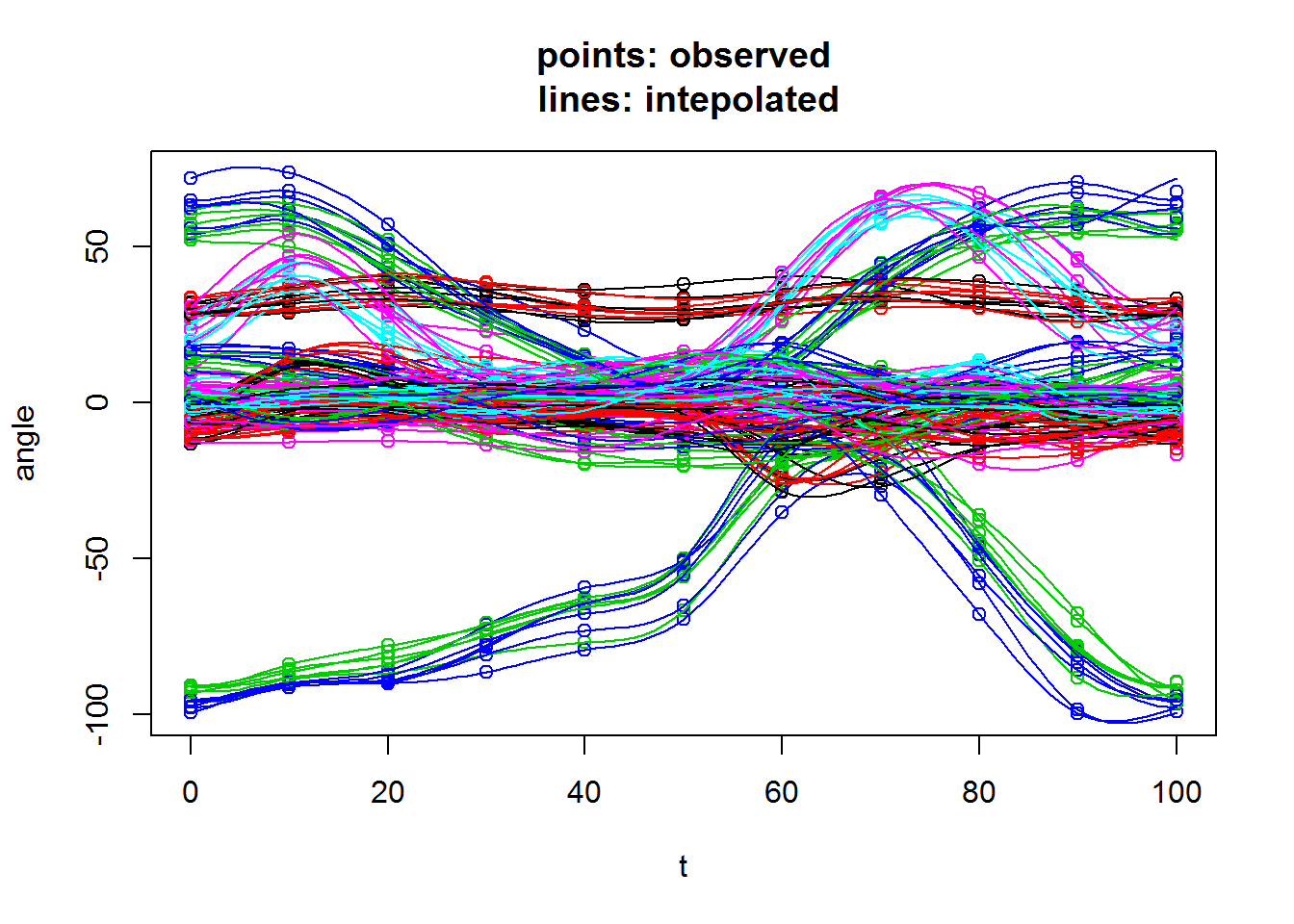
The plot=T argument plots the interpolated lines together with the observed points. It is recommended that you leave it as FALSE (default) if you are resampling many curves, because the plot will just be cluttered.